Enhancing a Package: Representing Uncertainty

Follow these steps to add realizations to a Package.

In the previous article, we added the ability to use timesteps in our models and graphically visualize the model outputs using charts. In this article, we will introduce Monte Carlo realizations for modelling uncertainty. The simulation is run for multiple iterations, and for each iteration, we will draw new values for the model calculations from a random distribution. The distribution parameters will be specified by the model inputs, so instead of directly specifying the slope, we will be specifying the mean and standard deviation of a normal distribution of slope values.

These enhancements will be part of a new Package, called helloworldUncertainty, within the helloworldEnhanced suite of Packages. This Package builds off the previous Package in the suite, helloworldTime. Follow these steps to set up this new Package:

Create a new subfolder within your working folder (e.g. c:\temp\helloworldUncertainty)
If creating a model in R, copy the package.xml and model.R files from the helloworldTime subfolder into the new helloworldUncertainty subfolder.
If creating a model in Python, copy the package.xml and model.py files from the helloworldTime subfolder into the new helloworldUncertainty subfolder.

Note

The final materials for this article can be downloaded using the following links:

R
- package.xml
- model.R
Python
- package.xml
- model.py

Step 1 - Add Iterations to the XML Configuration File

Note

The SyncroSim XML Package has the following structure:

XML version and Package name
Primary Transformer and Chart Transformer
Run Control
Model Inputs
Model Outputs
Layouts (Results Transformer, Library Datafeeds, Scenario Datafeeds, Charts)

Datafeeds and Datasheets

First, we need to add two new columns to the RunControl datafeed, named MinimumIteration and MaximumIteration. We will set the default values for the minimum and maximum number of iterations to "1" and "5", respectively, using the defaultValue attribute. The MinimumIteration column will also have the attribute isVisible="False". Since we know that the minimum number of iterations will always be 1, the user never has to set this value, so it is better to leave it out. This way we can also set the MaximumIteration column to be displayed as Number of Iterations. Here is the updated RunControl datafeed:

<!--Run Control-->
<datafeed name="RunControl" displayName="Run Control" dataScope="Scenario">
    <datasheets>
        <datasheet name="RunControl" displayName="Run Control" isSingleRow="True">
            <columns>
                <column name="RunControlID" dataType="Integer" isPrimary="True"/>
                <column name="ScenarioID" dataType="Integer"/>
                <column
                    name="MinimumIteration"
                    displayName="Minimum Iteration"
                    dataType="Integer"
                    defaultValue="1"
                    validationType="WholeNumber"
                    validationCondition="GreaterEqual"
                    formula1="1"
                    isVisible="False"/>
                <column
                    name="MaximumIteration"
                    displayName="Number of Iterations"
                    dataType="Integer"
                    defaultValue="5"
                    validationType="WholeNumber"
                    validationCondition="GreaterEqual"
                    formula1="1"/>
                <column
                    name="MinimumTimestep"
                    displayName="Minimum Timestep"
                    dataType="Integer"
                    defaultValue="0"
                    validationType="WholeNumber"
                    validationCondition="GreaterEqual"
                    formula1="0"/>
                <column
                    name="MaximumTimestep"
                    displayName="Maximum Timestep"
                    dataType="Integer"
                    defaultValue="10"
                    validationType="WholeNumber"
                    validationCondition="GreaterEqual"
                    formula1="0"/>
            </columns>
        </datasheet>
    </datasheets>
</datafeed>

We are now using the input values to specify the parameters of a random distribution rather than using the input values directly in the calculation. For this example, we will take slope values from a normal distribution, which is defined by mean and standard deviation parameters. Therefore, instead of having an m column in the input datasheet, we will have two new columns for mean and standard deviation: mMean and mSD. Here is the updated InputDatafeed:

<!--Model Inputs-->
<datafeed name="InputDatafeed" displayName="Inputs" dataScope="Scenario">
    <datasheets>
        <datasheet name="InputDatasheet" isSingleRow="True">
            <columns>
                <column name="InputDatasheetID" dataType="Integer" isPrimary="True"/>
                <column name="ScenarioID" dataType="Integer"/>
                <column name="mMean" dataType="Double" displayName="Slope Distribution Mean"/>
                <column 
                    name="mSD" 
                    dataType="Double" 
                    displayName="Slope Distribution Standard Deviation"/>
                <column name="b" dataType="Integer" displayName="Value for b"/>
            </columns>
        </datasheet>
    </datasheets>
</datafeed>

Lastly, we need to modify the OutputDatasheet. This tutorial relies on iterations to model uncertainty. Therefore, instead of hiding the Iteration column by setting the isOptional attribute to "True", we will remove the attribute all together. Here is the updated OutputDatafeed:

<!--Model Output-->
<datafeed name="OutputDatafeed" displayName="Outputs" dataScope="Scenario">
    <datasheets>
        <datasheet name="OutputDatasheet">
            <columns>
                <column name="OutputDatasheetID" dataType="Integer" isPrimary="True"/>
                <column name="ScenarioID" dataType="Integer"/>
                <column name="Iteration" dataType="Integer"/>
                <column name="Timestep" dataType="Integer" displayName="Timestep"/>
                <column name="y" dataType="Double" displayName="Value for y"/>
            </columns>
        </datasheet>
    </datasheets>
</datafeed>

In model.R, after loading the input datasheet, we need to extract the new model inputs. Add the following code to model.R:

# Extract model inputs from complete input dataframe
mMean <- myInputDataframe$mMean
mSD <- myInputDataframe$mSD
b <- myInputDataframe$b

In this example, we will use a for loop to sequentially run through each iteration of the simulation (more advanced R users may want to vectorize this process using map or apply functions). Because we are iteratively adding rows to our output dataframe, we need to define the empty myOutputDataframe before the for loop. Move the following code so that it appears just after we extract the model inputs:

# Setup empty R dataframe ready to accept output in SyncroSim datasheet format
myOutputDataframe <- datasheet(myScenario,
                               name = "helloworldEnhanced_OutputDatasheet")

Next, we will construct our for loop. Inside the for loop, we will still be using the linear equation y=mt+b, where t represents time. However, m is now a value taken from a normal distribution with mean mMean and standard deviation mSD. After this calculation, we will store the outputs in a temporary dataframe and append this dataframe to myOutputDataframe using the rsyncrosim addRow() function.

# For loop through iterations
for (iter in runSettings$MinimumIteration:runSettings$MaximumIteration) {
  
  # Extract a slope value from normal distribution
  m <- rnorm(n = 1, mean = mMean, sd = mSD)
  
  # Do calculations
  y <- m * timesteps + b
  
  # Store the relevant outputs in a temporary dataframe
  tempDataframe <- data.frame(Iteration = iter,
                              Timestep = timesteps, 
                              y = y)
  
  # Copy output into this R dataframe
  myOutputDataframe <- addRow(myOutputDataframe, tempDataframe)
}

In model.py, after loading the input datasheet, we need to extract the new model inputs. Add the following code to model.py:

# Extract model inputs from Input DataFrame
m_mean = my_input_dataframe.mMean.item()
m_sd = my_input_dataframe.mSD.item()
b = my_input_dataframe.b.item()

In this example, we will use a for loop to sequentially run through each iteration of the simulation (more advanced Python users may want to vectorize this process using the map function). Because we are iteratively adding rows to our output dataframe, we need to define the empty my_output_dataframe before the for loop. Move the following code so that it appears just after we extract the model inputs:

# Set up empty pandas DataFrame to accept output values
my_output_dataframe = myScenario.datasheets(name="helloworldEnhanced_OutputDatasheet")

Next, we will construct our for loop. Inside the for loop, we will still be using the linear equation y=mt+b, where t represents time. However, m is now a value taken from a normal distribution with mean m_mean and standard deviation m_sd. After this calculation, we will store the outputs in a temporary dataframe and append this dataframe to my_output_dataframe using the pandas append() function.

# For loop through iterations
for i in range(1, run_settings.MaximumIteration.item() + 1):
    
    # Extract a slope value from normal distribution
    m = np.random.normal(loc=m_mean, scale=m_sd)
    
    # Do calculations
    y = m * timesteps + b

    # Store relevant output in temporary data frame
    temp_data_frame = pd.DataFrame({"Timestep": timesteps,
                                    "Iteration": [i] * len(y),
                                    "y": y})

    # Append temporary data frame to output data frame
    my_output_dataframe = my_output_dataframe.append(temp_data_frame)

Step 3 - Rebuild the Package

Use the Package Manager to rebuild the Package using the new package.xml and model.R or model.py files shown above (see Step 4 in the Building a Package article).

Step 4 - Set Model Inputs

Start SyncroSim.
Create a new library based on the helloworldEnhanced Package.
Within the Library Properties, set the location of the R or Python executable in the R Configuration or Python Configuration tab.
Create a new Scenario - Right-click in the Library Explorer and select New > Scenario from the context menu. Rename this scenario to Timesteps with Uncertainty.
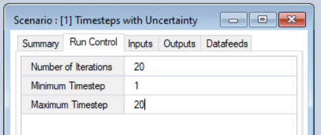
Edit the Scenario Run Control - Within the Timesteps with Uncertainty Scenario, navigate to the Run Control tab. Set the Number of Iterations, Minimum Timestep, and Maximum Timestep values for your model.

alt text

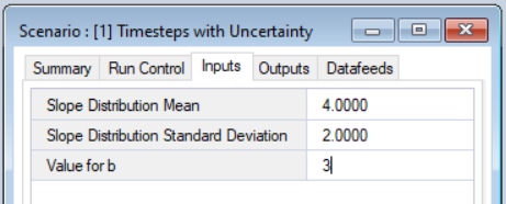
Edit the Scenario Inputs - Choose values for mMean, mSD, and b.

alt text

Save the Scenario inputs - Save changes made to the Scenario inputs.

Step 5 - Run the Model

Right-click on the Timesteps with Uncertainty Scenario in the Library Explorer and select Run to run this Scenario.

Step 6 - View the Results

Once the run is complete, return to the Library Explorer. Expand the node beside the Timesteps with Uncertainty scenario to reveal a Results folder containing your results, then expand the node beside the Results folder to show the newly generated date/time stamped Results Scenario. Each Results Scenario contains a read-only snapshot copy of all your inputs at the time of your run, along with values for your model generated outputs.

alt text

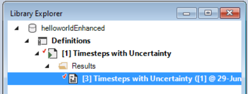
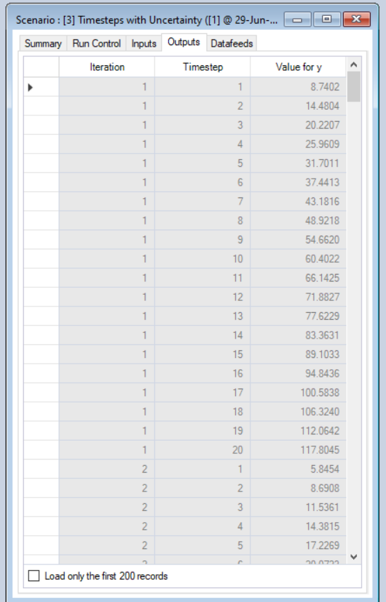
Right-click on this Results Scenario and select Properties to view the details of this Results Scenario; you will find your calculated outputs at each iteration and timestep under the Outputs tab.

alt text

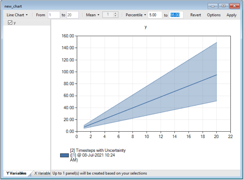
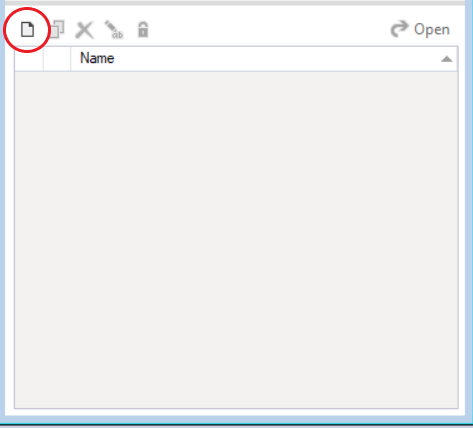
To graphically visualize the uncertainty, click on the Create a new chart button.

alt text

Fill in a name and select the y variable from the left panel. From the top toolbar, click on the dropdown menu title No Ranges, and select Percentile. In the boxes beside this dropdown, fill in the values "5" and "95". Click Apply to graphically view the change in y over time with 90% confidence intervals. To make further modifications to your chart, such as adding X and Y axes, see the Customizing a Chart tutorial.

alt text