Enhancing a Package: Adding Timesteps

Follow these steps to add timesteps and charts to a Package.

In the previous article we created a basic Package that performs a simple calculation. Now we will build on this basic Package by adding more advanced features. First, we will add a timestep feature so we can create models that vary over time. We will also add the ability to graphically visualize the model outputs using charts. For this example, we will model the change over time using a linear equation, y=mt+b, where t represents time.

These enhancements will be part of a new Package, called helloworldTime, within the helloworldEnhanced suite of Packages. Follow these steps to set up this new Package:

• Create a new subfolder within your working folder (e.g. c:\temp\helloworldTime)
• If creating a model in R, copy the package.xml and model.R files from the original helloworld subfolder into the new helloworldTime subfolder.
• If creating a model in Python, copy the package.xml and model.py files from the original helloworld subfolder into the new helloworldTime subfolder.

Note

The final materials for this article can be downloaded using the following links:

• R
  • package.xml
  • model.R
• Python
  • package.xml
  • model.py

Step 1 - Changing the Package Names

Before we start changing the files we copied from the helloworld subfolder, we will modify the package name in the XML file to helloworldEnhanced. All subsequent packages created in this tutorial series will also be called helloworldEnhanced.

<?xml version="1.0" encoding="utf-8"?>
<package name="helloworldEnhanced" displayName="Hello World Package Enhanced" version="1.0.0">

Datasheet names must also be changed in the model script. All names will hereafter begin with helloworldEnhanced to match the package name. For example, the input datasheet name will be changed to the following:

• R
• Python

# Load scenario's input datasheet from SyncroSim library into R dataframe
myInputDataframe <- datasheet(myScenario,
                              name = "helloworldEnhanced_InputDatasheet")

Step 2 - Add Timesteps to the XML Configuration File

Note

The SyncroSim XML Package has the following structure:

1. XML version and Package name
2. Primary Transformer and Chart Transformer
3. Run Control
4. Model Inputs
5. Model Outputs
6. Layouts (Results Transformer, Library Datafeeds, Scenario Datafeeds, Charts)

Transformers

Next, we must include a new Transformer within the Primary Transformer in the XML configuration file called corestime_Runtime. This Transformer uses the Runtime Transformer from the corestime built-in SyncroSim core to store chart information. The <include> tag tells the Package loader to reference Transformers in other Packages.

• R
• Python

<!--Primary Transformer-->
<transformer
    name="Primary"
    isPrimary="True"
    programName="Rscript"
    programArguments="model.R">

    <!--Chart Transformer-->
    <include>
        <transformer name="corestime_Runtime"/>
    </include>

    <datafeeds>

Datafeeds and Datasheets

To add timesteps, we will add a new Datafeed and Datasheet to our existing XML configuration file for the helloworld Package called RunControl. Since we want the user to be able to only input a single time series, we will force this datasheet to comprise only a single row using the isSingleRow attribute in the <datasheet> element. The new Datasheet needs two columns specifying the timestep range, called MinimumTimestep and MaximumTimestep. These new columns also have new attributes for ensuring the correct format and range of input data, defaultValue, validationType, validationCondition, and formula1. For more information on these new attributes, see the XML Reference. Here is the complete RunControl Datafeed to insert in package.xml:

<!--Run Control-->
<datafeed name="RunControl" displayName="Run Control" dataScope="Scenario">
    <datasheets>
        <datasheet name="RunControl" displayName="Run Control" isSingleRow="True">
            <columns>
                <column name="RunControlID" dataType="Integer" isPrimary="True"/>
                <column name="ScenarioID" dataType="Integer"/>
                <column
                    name="MinimumTimestep"
                    displayName="Minimum Timestep"
                    dataType="Integer"
                    defaultValue="0"
                    validationType="WholeNumber"
                    validationCondition="GreaterEqual"
                    formula1="0"/>
                <column
                    name="MaximumTimestep"
                    displayName="Maximum Timestep"
                    dataType="Integer"
                    defaultValue="10"
                    validationType="WholeNumber"
                    validationCondition="GreaterEqual"
                    formula1="0"/>
            </columns>
        </datasheet>
    </datasheets>
</datafeed>

Since we are modelling a linear equation that varies with time, we will update the names of our input variables from x and a to m and b. The input datasheet will also consist of a single row, as designated by the isSingleRow attribute, because we only want to specify the input values once. Here is the updated InputDatafeed in package.xml:

<!--Model Inputs-->
<datafeed name="InputDatafeed" displayName="Inputs" dataScope="Scenario">
    <datasheets>
        <datasheet name="InputDatasheet" isSingleRow="True">
            <columns>
                <column name="InputDatasheetID" dataType="Integer" isPrimary="True"/>
                <column name="ScenarioID" dataType="Integer"/>
                <column name="m" dataType="Double" displayName="Value for m"/>
                <column name="b" dataType="Integer" displayName="Value for b"/>
            </columns>
        </datasheet>
    </datasheets>
</datafeed>

Finally, to see the output values at the end of each timestep, we need to add Timestep and Iteration columns to the OutputDatasheet. Although we will not be using iterations in this tutorial, the Iteration column is required by the built-in charting software. We will revisit setting iterations for modelling uncertainty in the next article. This column also has a new attribute called isOptional. By default, all columns after ScenarioID are displayed in the SyncroSim Windows Interface. When isOptional is set to "True", the column is hidden unless manually inserted by the user. Here is the updated OutputDatasheet in package.xml:

<!--Model Output-->
<datafeed name="OutputDatafeed" displayName="Outputs" dataScope="Scenario">
    <datasheets>
        <datasheet name="OutputDatasheet">
            <columns>
                <column name="OutputDatasheetID" dataType="Integer" isPrimary="True"/>
                <column name="ScenarioID" dataType="Integer"/>
                <column name="Iteration" dataType="Integer" isOptional="True"/>
                <column name="Timestep" dataType="Integer"/>
                <column name="y" dataType="Double" displayName="Value for y"/>
            </columns>
        </datasheet>
    </datasheets>
</datafeed>

Layouts

To add charting capability to our Package, we need to add two new layouts to the configuration file. The first layout, named coreforms_ResultTransformers, creates the result panel in the bottom left-hand corner of the SyncroSim Windows Interface. The second layout, named corestimeforms_Charts indicates which data from the specified datasheets will be used in this chart display. This data will show up in the left-hand criteria window when creating a new chart. This second new layout also contains an attribute called configurationSheet, which is set to the RunControl datafeed. This attribute ensures the charting software recognizes the Timestep column in the RunControl datafeed and adds plotting functionality based on this column.

The final step in updating the XML configuration file involves adding the new RunControl Datafeed to the Scenario Datafeeds Layout. Here is the updated layout in package.xml:

• R
• Python

<layouts>

    <!--Results Transformer Layout-->
    <layout name="coreforms_ResultTransformers">
        <item name="corestime_ChartTransformer"/>
    </layout>

    <!--Library Datafeeds Layout-->
    <layout name="coreforms_LibraryDatafeeds">
        <item name="core_Rconfig"/>
    </layout>

    <!--Scenario Datafeeds Layout-->
    <layout name="coreforms_ScenarioDatafeeds">
        <item name="RunControl"/>
        <item name="InputDatafeed"/>
        <item name="OutputDatafeed"/>
    </layout>

    <!--Charts Layout-->
    <layout name="corestimeforms_Charts" configurationSheet="RunControl">
        <item name="y" displayName="y" dataSheet="OutputDatasheet" column="y"/>
    </layout>

</layouts>

Step 3 - Modify the Model Script

• R
• Python

You will now need to modify the R script from the previous article to incorporate timesteps. First, we load the new RunControl Datasheet into a variable called "runSettings". Then we create a vector of timesteps based on the maximum and minimum specified by the user.

# Load RunControl datasheet to be able to set timesteps
runSettings <- datasheet(myScenario, name = "helloworldEnhanced_RunControl")

# Set timesteps - can set to different frequencies if desired
timesteps <- seq(runSettings$MinimumTimestep, runSettings$MaximumTimestep)

Next, we will load the model inputs, extract the slope (m) and intercept (b), and apply the linear equation that varies with time.

# Load scenario's input datasheet from SyncroSim library into R dataframe
myInputDataframe <- datasheet(myScenario,
                              name = "helloworldEnhanced_InputDatasheet")

# Extract model inputs from complete input dataframe
m <- myInputDataframe$m
b <- myInputDataframe$b

# Do calculations
y <- m * timesteps + b

Finally, the y value corresponding to each timestep is added to the output dataframe, and the final output is saved.

# Setup empty R dataframe ready to accept output in SyncroSim datasheet format
myOutputDataframe <- datasheet(myScenario,
                               name = "helloworldEnhanced_OutputDatasheet")

# Copy output into this R dataframe
myOutputDataframe <- data.frame(Timestep = timesteps, y = y)

# Save this R dataframe back to the SyncroSim library's output datasheet
saveDatasheet(myScenario,
              data = myOutputDataframe,
              name = "helloworldEnhanced_OutputDatasheet")

Step 4 - Rebuild the Package

Use the Package Manager to rebuild the Package using the new package.xml and model.R or model.py files shown above (see Step 4 in the Building a Package article).

Step 5 - Set Model Inputs

1. Start SyncroSim.
2. Create a new library based on the helloworldEnhanced Package.
3. Within the Library Properties, set the location of the R or Python executable in the R Configuration or Python Configuration tab.
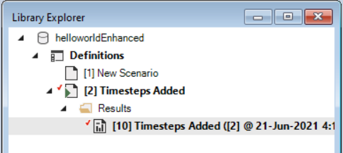
4. Create a new Scenario - Right-click in the Library Explorer and select New > Scenario from the context menu. Rename this scenario to Timesteps Added.
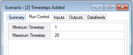
5. Edit the Scenario Run Control - Within the Timesteps Added Scenario, navigate to the Run Control tab. Set the Minimum Timestep and Maximum Timestep values for your model.

6. Edit the Scenario inputs - In the Inputs tab, specify input values for the slope (m) and intercept (b) of the linear equation.

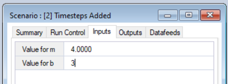
7. Save the Scenario inputs - Save changes made to the Scenario inputs.

Step 6 - Run the Model

Right-click on this Timesteps Added Scenario again in the Library Explorer and select Run to run this Scenario.

Step 7 - View the Results

1. Once the run is complete, return to the Library Explorer. Expand the node beside the New Scenario to reveal a Results folder containing your results, then expand the node beside the Results folder to show the newly generated date/time stamped Results Scenario. Each Results Scenario contains a read-only snapshot copy of all your inputs at the time of your run, along with values for your model generated outputs.

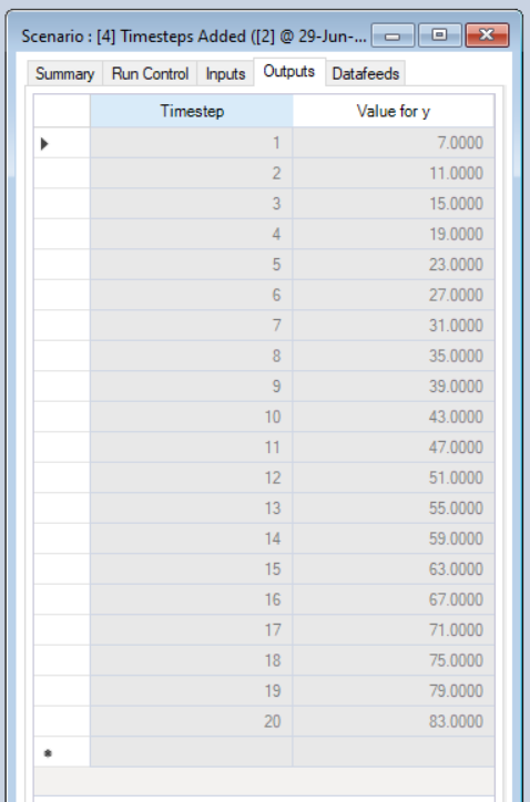
2. Right-click on this Results Scenario and select Properties to view the details of this Results Scenario; you will find your calculated outputs at each timestep under the Outputs tab.

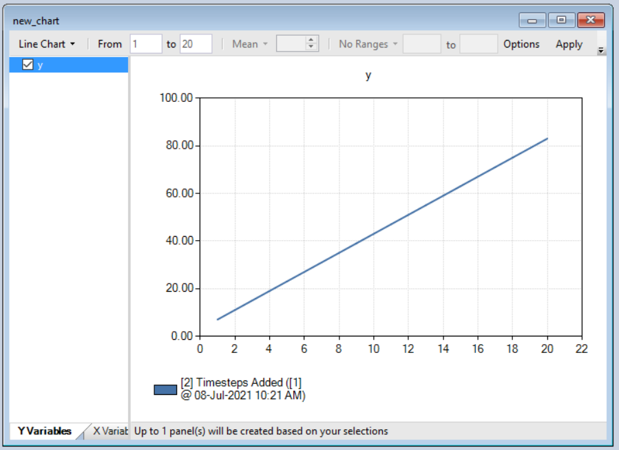
3. In the bottom left-hand corner, a Results Viewer should now be visible with a Charts tab. Within this viewer, click on the Create a new chart button.

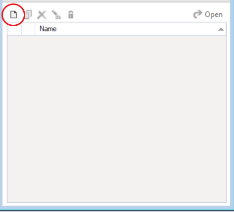
4. Fill in a name, select the y variable from the left panel, and click Apply to graphically view the change in y over time. To make further modifications to your chart, such as adding X and Y axes, see the Customizing a Chart tutorial.